Example 002: Extrapolation of simulation data
import numpy as np
import matplotlib.pyplot as plt
import iddefix
from scipy.constants import c
Simulation data example
This example features CST simulated wakefield data of the “Accelerator Cavity” introductory example.

Fitting on fully decayed wakefield
Import data
# Importing impedance data
data_fully_decayed = np.loadtxt(
    "examples/data/002_impedance_acceleratorCavity_fully_decayed.txt",
    comments="#",
    delimiter="\t",
)

# Extracting frequency and impedance

frequency = data_fully_decayed[:, 0] * 1e9  # Convert to GHz
real_impedance = data_fully_decayed[:, 1]
imag_impedance = data_fully_decayed[:, 2]

impedance_fd = real_impedance + 1j * imag_impedance
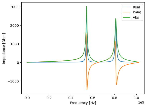
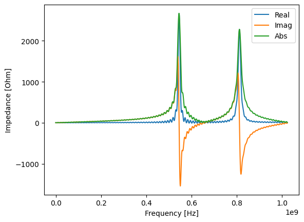
Visually inspecting the impedance
plt.plot(frequency, impedance_fd.real, label="Real")
plt.plot(frequency, impedance_fd.imag, label="Imag")
plt.plot(frequency, np.abs(impedance_fd), label="Abs")

plt.xlabel("Frequency [Hz]")
plt.ylabel("Impedance [Ohm]")
plt.legend()
<matplotlib.legend.Legend at 0x7f797cbb0f50>
Fitting resonators with IDDEFIX on the absolute magnitude of the 3 resonator impdance spectrum
# Setting amount of resonators to fit
N_resonators = 2
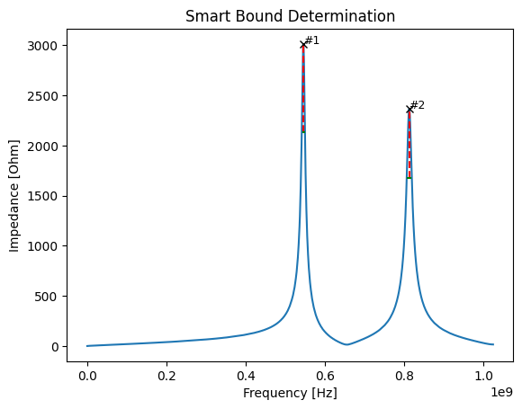
# Bounds on resonators parameters
""" In this example, we will use the SmartBoundDetermination class to determine the bounds on the resonators parameters.
By using SmartBoundDetermination ther is no need to specify the bounds manually."""
SBD_parameterBound = iddefix.SmartBoundDetermination(
frequency, np.abs(impedance_fd), minimum_peak_height=1000
)
SBD_parameterBound.inspect()
Running IDDEFIX DE
Running the DE algorithm with IDDEFIX and chosen parameters.
%%time
DE_model_fd = iddefix.EvolutionaryAlgorithm(
    frequency,
    impedance_fd,
    N_resonators=N_resonators,
    parameterBounds=SBD_parameterBound.find(),
    plane="longitudinal",
    objectiveFunction=iddefix.ObjectiveFunctions.sumOfSquaredError,
)

DE_model_fd.run_differential_evolution(
    maxiter=30000, popsize=30, tol=0.01, mutation=(0.4, 1.0), crossover_rate=0.7
)
print(DE_model_fd.warning)
Optimization Progress %: 0%| | 0/100 [00:00<?, ?it/s]
Optimization Progress %: 112.70799498485952it [00:07, 14.96it/s]
----------------------------------------------------------------------
Resonator |   Rs [Ohm/m or Ohm]    |        Q         |    fres [Hz]
----------------------------------------------------------------------
    1     |        3.04e+03        |      69.97       |    5.453e+08
    2     |        2.37e+03        |      64.96       |    8.123e+08
----------------------------------------------------------------------
callback function requested stop early
CPU times: user 3.44 s, sys: 2.13 s, total: 5.57 s
Wall time: 7.58 s
Minimization step
To further refine the solution obtained by the DE algorithm, a second optimization step is applied using the Nelder-Mead minimization algorithm.
DE_model_fd.run_minimization_algorithm()
Method for minimization : Nelder-Mead


----------------------------------------------------------------------
Resonator |   Rs [Ohm/m or Ohm]    |        Q         |    fres [Hz]
----------------------------------------------------------------------
    1     |        3.03e+03        |      69.88       |    5.453e+08
    2     |        2.36e+03        |      64.55       |    8.123e+08
----------------------------------------------------------------------
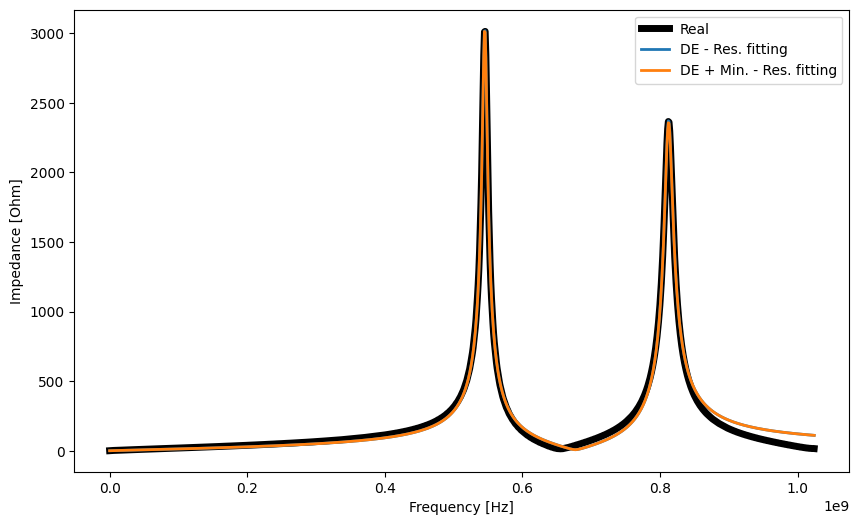
Assesing the fitting visually
plt.figure(figsize=(10, 6))
result_DE = np.abs(DE_model_fd.get_impedance(use_minimization=False))
result_DE_MIN = np.abs(DE_model_fd.get_impedance())

plt.plot(frequency, np.abs(impedance_fd), lw=5, label="Real", color="black")
plt.plot(frequency, result_DE, lw=2, label="DE - Res. fitting")
plt.plot(frequency, result_DE_MIN, lw=2, label="DE + Min. - Res. fitting")
plt.xlabel("Frequency [Hz]")
plt.ylabel("Impedance [Ohm]")
plt.legend()
<matplotlib.legend.Legend at 0x7f79a89217d0>
Fitting on partially decayed wakefield
Import data
# Importing impedance data
data_partially_decayed = np.loadtxt(
    "examples/data/002_impedance_acceleratorCavity_partially_decayed.txt",
    comments="#",
    delimiter="\t",
)

# Extracting frequency and impedance

frequency = data_partially_decayed[:, 0] * 1e9  # Convert to GHz
real_impedance = data_partially_decayed[:, 1]
imag_impedance = data_partially_decayed[:, 2]

impedance_pd = real_impedance + 1j * imag_impedance
Visually inspecting the impedance
plt.plot(frequency, impedance_pd.real, label="Real")
plt.plot(frequency, impedance_pd.imag, label="Imag")
plt.plot(frequency, np.abs(impedance_pd), label="Abs")

plt.xlabel("Frequency [Hz]")
plt.ylabel("Impedance [Ohm]")
plt.legend()
<matplotlib.legend.Legend at 0x7f7991f86890>
Fitting resonators with IDDEFIX
# Setting amount of resonators to fit

N_resonators = 2

# Bounds on resonators parameters
""" Bounds have this format [(Rs_min, Rs_max), (Q_min, Q_max), (fres_min, fres_max)].
ParameterBounds allows us to manually add a resonator with desired parameters """

bounds = [
    (1e3, 1e4),
    (1, 1e3),
    (0.4e9, 0.9e9),
]  # Bounds have this format [(Rs_min, Rs_max), (Q_min, Q_max), (fres_min, fres_max)].
parameterBounds = N_resonators * bounds
Running IDDEFIX DE
Running the DE algorithm with IDDEFIX and chosen parameters.
%%time
DE_model_pd = iddefix.EvolutionaryAlgorithm(
    frequency,
    impedance_pd,
    N_resonators=N_resonators,
    parameterBounds=parameterBounds,
    plane="longitudinal",
    wake_length=25.4,
    objectiveFunction=iddefix.ObjectiveFunctions.sumOfSquaredError,
)

DE_model_pd.run_differential_evolution(
    maxiter=30000, popsize=30, tol=0.01, mutation=(0.4, 1.0), crossover_rate=0.7
)
print(DE_model_pd.warning)
Optimization Progress %: 110.93788471285839it [00:09, 12.05it/s]
----------------------------------------------------------------------
Resonator |   Rs [Ohm/m or Ohm]    |        Q         |    fres [Hz]
----------------------------------------------------------------------
    1     |        3.06e+03        |      71.98       |    5.452e+08
    2     |        2.34e+03        |      64.35       |    8.123e+08
----------------------------------------------------------------------
callback function requested stop early
CPU times: user 6.08 s, sys: 4.4 s, total: 10.5 s
Wall time: 9.24 s
Minimization step
DE_model_pd.run_minimization_algorithm()
Method for minimization : Nelder-Mead


----------------------------------------------------------------------
Resonator |   Rs [Ohm/m or Ohm]    |        Q         |    fres [Hz]
----------------------------------------------------------------------
    1     |        3.05e+03        |      71.79       |    5.453e+08
    2     |        2.36e+03        |      64.98       |    8.123e+08
----------------------------------------------------------------------
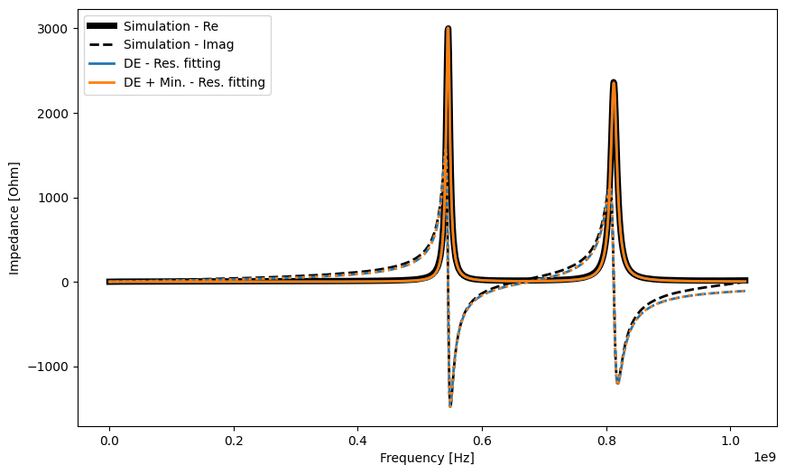
Assesing the fitting visually
plt.figure(figsize=(10, 6))
result_DE = DE_model_pd.get_impedance(use_minimization=False)
result_DE_MIN = DE_model_pd.get_impedance()

plt.plot(frequency, np.real(impedance_fd), lw=5, label="Simulation - Re", color="black")
plt.plot(
    frequency,
    np.imag(impedance_fd),
    lw=2,
    ls="--",
    label="Simulation - Imag",
    color="black",
)
plt.plot(
    frequency, np.real(result_DE), lw=2, label="DE - Res. fitting", color="tab:blue"
)
plt.plot(frequency, np.imag(result_DE), lw=2, ls="--", color="tab:blue")
plt.plot(
    frequency,
    np.real(result_DE_MIN),
    lw=2,
    label="DE + Min. - Res. fitting",
    color="tab:orange",
)
plt.plot(frequency, np.imag(result_DE_MIN), lw=2, ls=":", color="tab:orange")
plt.xlabel("Frequency [Hz]")
plt.ylabel("Impedance [Ohm]")
plt.legend()
<matplotlib.legend.Legend at 0x7f79a8a05510>
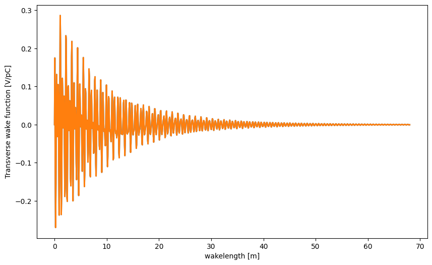
Having fitted the resonators, we are also able to produce the wake function for any given wakelength:
plt.figure(figsize=(10, 6))

timeframe = np.linspace(0, 68, 1000) / c

# From the formulas in resonatorFormalism.py
wake_function = (
    iddefix.Wakes.n_Resonator_longitudinal_wake(
        timeframe, DE_model_pd.minimizationParameters
    )
    / 1e12
)

# Or from the DE class itself:
wake_function_bis = DE_model_pd.get_wake(timeframe) / 1e12

plt.plot(timeframe * c, wake_function, lw=2, label="DE - Res. fitting")
plt.plot(
    timeframe * c,
    wake_function_bis,
    lw=2,
)
plt.xlabel("wakelength [m]")
plt.ylabel("Transverse wake function [V/pC]")
Text(0, 0.5, 'Transverse wake function [V/pC]')